Robot position calculation - using simplified Filter-Smoother

Every popular robotics or micro-controller forum has a thread where people argue if commanded motor power level linearly translates to motor speed, force, or something else.

The correct answer to this question is: it depends. It depends on many things.

https://vexforum.com/attachment.php?attachmentid=9621&stc=1&d=1444196372

Each motor has a nominal (or idle/no load) speed. Even without load it still draws some current (consumes some power). It spends it to counteract whatever little friction its gears have and heats up its electromagnet coil a bit because the wire has non-zero electric resistance.

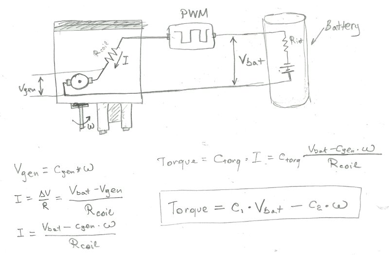
When motor’s rotor spins at a speed (w) it acts as a little electrical generator that would produce Vemf = Vgen, which is just slightly less than battery voltage Vbat, and we would get some small current going through its Rcoil from higher to lower potential. The power converted to mechanical energy is Vgen*I and the power to heat coil is (Vbat-Vgen)*I. Eventually all that energy will convert to heat.

Alternative way of thinking may be that to counteract friction in the motor you need specific Torque, which has linear relationship with the electric current (via some Ctorq coefficient for this particular motor). Once you know the current you will know voltage drop over the motor’s internal resistance Rcoil and then the motor could speed up up to speed (w) that corresponds to Vemf=Vgen via some constant Cgen, until Vemf matches remaining voltage differential (Vbat-Rcoil*I).

One way or another, for each load (torque) and supply voltage (Vbat) motor settles on a speed (w), see 393 motor curves. The important result is that without PTC kicking in we expect linear relationship between torque, Vbat, and w (Torque = C1 * Vbat - C2 * w) where C1 and C2 some coefficients for our specific motor. To keep our formulas simple and motors running all the time it is a good idea to manage motor load to prevent PTCs from tripping anyways.

Now we have to consider effects of PWM. Essentially, motor controller connects motor to the power supply Vbat for only a fraction of the time. One way of thinking about it that you still could have full force (Vbat) but have current flowing only part of the time, thus getting access to a fraction of the max power. However, since motor rotor’s moment of inertia acts as a mechanical capacitor that smoothes voltage=0 and voltage=Vbat periods into an average effective voltage we could say that we have access to the fraction of the supply voltage Vbat corresponding to the duty cycle.

According to this thread MC29 has non-linear relationship between commanded power level and actual output power level. Here is an example from VEXPro thread. Turned out that VEXPro was actively monitoring motor speed and throttling motor power to achieve linear relationship, while MC29 was letting laws of physics inside its less than perfect circuit with simple firmware define the shape of the curve:

https://vexforum.com/attachment.php?attachmentid=6136&d=1337552779

To make things more interesting for us here is a quote from Paul:

So, you may in fact find that your old MC29 will behave differently from the version with the newer firmware.

However, if you know exact parameters of the specific hardware pieces you have, it shouldn’t matter. The curve shape is predictable and known. If we create a lookup table (or try to fit a polynomial) between commanded and actual values we will know the effective voltage supplied to the motor at all the times.

Since we can estimate the speed of each motor, and we know commanded motor voltage - we can calculate output torque and, therefore, predict acceleration and the future path of the robot. The takeaway is that MC29 non-linear curve requires some additional coding and testing from us, but is not a showstopper at all.
While fixing a broken link in the previous post, I realized how easy it was to get lost in a few important motor related threads on this forum. Here is a single table listing those threads and direct links to some of the key posts:

jpearman: Motor torque-speed curves (70588) (linear speed graph)

jpearman: cortex motor speed testing (71992) (Paul’s non-linear quote)

jpearman: VEXpro motor speed tests (71995)

jpearman: estimating motor current (72100) (Code to detect PTC tripping) (official stall charts)

jpearman: Motor torque-speed curves - REV2 (73273) (motor curves graph) (PTC thermal image)

vamfun: Estimating 269 Motor Current based on H bridge models (73318) (firmware versions quote) (results and C code)

vamfun: Smart software monitor keeps PTC fuses from tripping (73960)

jpearman: estimating motor current - part 3 (74594)

jpearman: Smart Motor Library (74659) (TLD) (latest version at GitHub - jpearman/smartMotorLib)

LegoMindstormsmaniac: 24C’s Motor Control Value Remapping (76943)

The old VEXPro controlled its H-Bridge in a different way to the cortex and MC29 (higher pwm frequency and brake during “off” period rather than coast. That’s the reason for the linear responce. It did have the ability to determine motor velocity using back-emf, but that was not used as part of the motor drive control loop IIRC.

Interesting
 I guess, I misread the original thread then.

Do you know if there were any visible changes associated with the promised controller firmware update? After reading the old threads it feels like you need to test every piece of hardware you have in order to avoid interesting surprises.

I am still figuring out how to present object motion under influence of off-center forces without matrix math and lots of fancy greek symbols that are taught in college. Then there is similar problem with filter-smoother itself. Is it even possible to implement get it going without matrix operations such as matrix inversion - I certainly hope so.

In any case, here is a simple example:

Consider already familiar two-wheeled “turtlebot” that we are going to drive straight forward with equal power commanded to both motors. Its center of gravity will experience acceleration from combined force from both motors minus force of friction:

[INDENT]a = F/m = (Fmotor- Ffriction) / m = (2Torquew*wheel_radius - Ffriction) / m. [/INDENT]

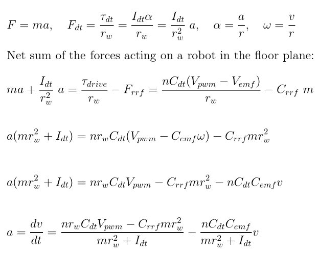
Substituting with relationships from the earlier post we could write:

[INDENT]a(t) = Cpower_coefficient * Vpwm - Cfriction_losses - Cemf * current_instanteneous_velocity(t)[/INDENT]

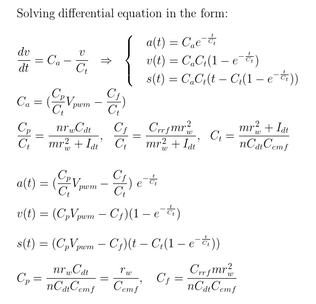
Then after sparing you from solving differential equation for a = dv/dt the resulting formulas for predicted a(t), v(t), and s(t) for acceleration, velocity, and driven distance as functions of time are:

[INDENT]a(t) = (CpVpwm - Cf) * exp(-t/Ct)
v(t) = (Cp
Vpwm - Cf) * Ct * ( 1 - exp(-t/Ct) )
s(t) = (Cp*Vpwm - Cf) * Ct * ( t - Ct *(1 - exp(-t/Ct) ) )[/INDENT]

Where:

[INDENT]Vpwm is the effective voltage coming from the PWM controller output (in case of MC29 commanded power needs to be linearized).

Cp is a power coefficient depending on drivetrain layout, motor specifications, and robot mass.
Cf is some coefficient corresponding to aggregate power losses due to drivetrain friction and rolling resistance.
Ct is some other coefficient corresponding to how fast the robot of a given mass will accelerate with this drivetrain configuration.
[/INDENT]
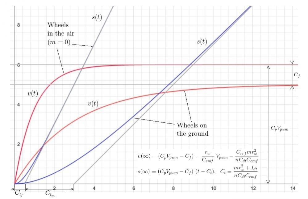
If you pull out your graphing calculators you will see that those are exponential curves similar to the capacitor charge-discharge graphs and are frequently seen by engineers.

All three coefficients are found experimentally using null test cases, that Collin is doing, and are applicable for the specific robot of mass m, configured and driven in a certain drivetrain configuration. If you significantly change robot mass, lubricate or replace motors, or change the wheels you may need to recalibrate your coefficients. However, after minor changes or tweaks the filter (or post-process run on logged residuals) will be able to estimate correction to those coefficients just by doing a few driving passes and turns.

Those who want to implement filter-smoother algorithm for their robot navigation, could start implementing precision measurement task as outlined in post #16. Next, we will define the methodology for finding calibration coefficients and will be able to do some runs and compare predicted and observed sensor measurements.

These solutions assume that Vpwm acts as a step input, correct? If Vpwm is some other function of time (ramp, sinusoidal, unknown, etc) then the solution could be drastically different (and potentially unstable in cases other than a drive system). That is something you may need to keep in mind as you progress further.

I can’t say I’m proficient, or even competent in any manner in Physics, but current is d/dt(charge), so if the current is velocity, then the integral of current, charge, would be the distance.

Yes, you are correct!

That’s what it looks like if we start drawing analogies. It is very tempting to say that when we apply voltage to the motors we start “charging” our mechanical system with kinetic energy and robot itself going with the speed (v) acts as a large capacitor or accumulator, while motor’s rotor, gears, and wheels rotating at various angular velocities (w) store smaller amount of energy acting like smaller filter caps. :slight_smile:

But then we start talking about real capacitors in VEX electric components and it all becomes very confusing.

Thank you for looking at this tutorial with a critical eye. I agree - there are many assumptions here.

Essentially, I looked at images in 71992 and concluded that it would be safe to assume square PWM output.

I didn’t want to overwhelm anyone, including myself, with extra details so there is a number of other things there were left out in this example. Later when we write actual path inegrator we may choose to include modeling for some of the more advanced steps.

But for now the assumption is that we don’t gradually increase commanded power and there is no initial motor jerk due to motor gear slop or static friction coefficient. There is no consideration of internal battery resistance and any of the PTCs that the current will flow through, neither there is any modeling of the motor’s coil inductance or capacitance in the circuit.

Essentially, for solving motion equations we assume that once PWM is commanded to certain power level its effective output voltage will remain constant throughout the integration step. Also, we assume that aggregate friction losses due to drivetrain kinetic friction coefficient and rolling resistance coefficient are both constant and independent of the robot velocity. They only depend on drivetrain configuration and linearly proportional to the robot mass, which we assume to stay constant as well.

Hers is a graph from a paper by Dr. RaĂșl Rojas of FU-Fighters:

https://vexforum.com/attachment.php?attachmentid=9630

As you can see acceleration of the motor driven by PWM follows quite complex path but if we “zoom out” it will look like an exponential function. VEX robots tend to be heavy and PWM frequency is high (1200Hz) so most of the PWM pulsing will be absorbed by the drivetrain inertia. In addition to that, we will have non-zero sigma error bounds for our quad encoder measurements that should comfortably absorb any leftover oscillations.
rojas_pwm_acceleration.jpg

I thoroughly enjoy reading this thread and check back often to see your progress. Controls as a whole isn’t usually discussed in detail on the forum beyond PID loops, so this thread is really exciting (because plant/system modeling is the basis of every controls problem).

I like saying that engineering is just the art of taking physics and making assumptions to get just “good enough” results. One difference between good engineering and bad engineering is the proper or improper use of assumptions and if one can tell what is really “good enough.”

So far, the assumptions I’ve seen in this thread seem fine. It all comes down to the required precision of the robot position calculation. If the launcher only requires knowing the robots position within an inch and the objects on the field are placed within an inch, there isn’t much use in knowing the position of the robot to the millimeter (something you mentioned before about EKFs)

Once I get a copy of RobotC available, I can try to do a few tests. I was thinking about recording the encoder response to a control value step input and using the data to generate the plant model in MatLAB. I’m curious to see what order model is the best fit.

The transfer function from a voltage input to the angular velocity or position output of the motor isn’t to difficult. The part I have had trouble figuring out is the transfer function of a control value input to a voltage output from the DC side of the MC29. I figure an experimental model will probably be better than any theoretical model I try to develop.

We already know that predicted motion of our robot going straight forward will be:

[INDENT]a(t) = (CpVpwm - Cf) * exp(-t/Ct)
v(t) = (Cp
Vpwm - Cf) * Ct * ( 1 - exp(-t/Ct) )
s(t) = (Cp*Vpwm - Cf) * Ct * ( t - Ct *(1 - exp(-t/Ct) ) )[/INDENT]

Where:

[INDENT]Vpwm is the effective voltage output from the PWM controller (in case of MC29 relation between commanded power and output voltage is non-linear). We assume it doesn’t change during our experiment.
[/INDENT]
And experimentally determined coefficients (for our specific robot with mass m=1):
[INDENT]Cp is a power coefficient depending on drivetrain layout and motor specifications.
Cf is some coefficient corresponding to power losses due to drivetrain friction and rolling resistance.
Ct is some other coefficient corresponding to how fast our robot will accelerate in this drivetrain configuration.
[/INDENT]

The graph for the velocity will look like this:

https://vexforum.com/attachment.php?attachmentid=9630

If you read Dr. Rojas’ paper, you would guess that when robot is turning in place (wheels driving in the opposite directions) then its angular velocity, acceleration, and heading would have very similar formulas.

So here is a question / homework:

How should we change the formulas if the robot mass doubles?

You don’t have to give the exact formulas, just offer us some reasoning. And, yes, it is a tricky question but there will be prizes for active participation.

Ct would be at half of its old value because it would take twice as much force to accelerate the robot the same amount as before (a=f/m, a=f/2m, 1/2=f/m)

We also might expect that a greater weight of the robot will cause its wheels to sink more into the foam tiles, as you pointed out in one of your previous posts, which might increase friction, meaning we’d need to increase Cf to account for it.

Your reasoning about considering rolling resistance and Newton’s law is correct, but numerical conclusions are not. I said it is a trick question, because at the first glance the answer is totally counter-intuitive.

Try to consider edge cases when t=0 and t is large enough so that exp(-t/Ct) is practically zero. What would you expect acceleration and velocity to be in those cases? How exactly does rolling resistance depends on the mass?

You are definitely in the running for the prizes.

Well I will take a shot at the homework I suppose.

I am going to work with the acceleration equation here for simplicity. First we consider the robot at t=0 without any friction. That reduces this equation to:

Now from Newton’s third law, we expect the initial acceleration of the robot with double the mass to be half of that of the original because the force applied by the motors should be the same. Therefore, we would expect Cp be halved.

Next, we should look at the force due to friction. Again we will assume t-0.

As Bpalms said, one would expect the friction of the heavier robot to be greater than the lighter one. Friction is a complicated subject (especially the friction between a rigid and semi-rigid surface). As such, I do not feel comfortable giving any magnitude of the expected change. Based on this, the Cf constant should increase by some amount.

The final piece is to consider Ct. This constant determines how long it takes the robot to reach top speed. This is the part that may be the least intuitive. One would expect a heavier robot to take longer to accelerate to top speed, and this is correct. However, we can see that the only time dependent part of the acceleration is the exponential function:

This exponential function starts out as 1 (when t=0) and approaches 0 as t goes to infinity. If we want this process to slow down, we must increase the Ct coefficient. Since t is divided by Ct, if we double Ct then it will take twice as long for the exponential function to reach 0. We can say that this coefficient will roughly double because Ct is a function of polar moment of inertia (of which is linear function of mass).

To summarize, if the mass doubles:
Cp will be roughly halved
Cf will be increases by some amount
Ct will be roughly doubled

I say roughly because there are some linear assumption in the background that may or may not be true. In the regime these robots operate, I would hazard these assumption are pretty good.

Hopefully I didn’t make any silly mistakes.

Yes, this agrees with my estimates. The most counter-intuitive part is Cf.

Friction losses come from the following components:

Force of rolling resistance in floor tiles, tires, and weight bearing (adj) bearings (noun) which is proportional to the mass of the robot:
[INDENT] Frr = Crr1 * Fnormal = Crr1 * mg = Crr * m
[/INDENT]

Force of kinetic friction in drivetrain gear teeth, sprokets, and axles depends on Fnormals which proportional to the transmitted drive force:
[INDENT] Fdtf = Cdtf1 * MotorOutputTorque = Cdft1 * Fdrive / wheel_radius = Cdtf * Fdrive
[/INDENT]

This lets us write Newton’s Law formula as:
[INDENT]ma = (Fdrive - Ffriction) = (Fdrive - Fdtf - Frr)
ma = Fdrive - CdfFdrive - Crr * m
ma = Fdrive * (1-Cdtf) - Crr * m
ma = C1
(Vpwm - Vemf)(1 - Cdtf) - Crrm
ma = C1*(1-Cdtf) * Vpwm - C1*(1-Cdtf)Vemf - Crrm
ma = C1*(1-Cdtf) * Vpwm - C1*(1-Cdtf)C2velocity - Crr*m

a = (C1*(1-Cdtf)/m) * Vpwm - (C1*(1-Cdtf)*C2/m)*velocity - Crr

a = dv/dt = (C3/m) * Vpwm - (C4/m) * v - Crr
[/INDENT]
Solving this differential equation will lead to a familiar formulas:
[INDENT]a(t) = ((Cp/m)Vpwm - Cf) * exp(-t/(mCt))
v(t) = ((Cp/m)Vpwm - Cf) * mCt * ( 1 - exp(-t/(mCt)) )
s(t) = ((Cp/m)Vpwm - Cf) * mCt * ( t - m
Ct (1 - exp(-t/(mCt)) ) )
[/INDENT]
Essentially, Cp and Ct have absorbed Cdtf (kinetic friction coefficients in the drivetrain). While Cf absorbed all rolling resistance coefficients and kinetic friction coefficient between wheel axles and weight bearing bearings (where friction is proportional to the robot mass).

An intuitive explanation to this may be that since Cf signifies power losses then it should not decrease as the robot mass increases.

At the end of the day Cf will roughly stay the same. Finding analytical formulas without any “roughlys” is beyond my expertise in solving partial differential equations so we will depend on filter to smooth out any rough approximations.

And now another tricky question: What will happen to the formulas if we double number of our drivetrain motors while everything else stays the same?

As engineers we could be cavalier about roughness of our coefficients while adding new motors but we will certainly remove some metal to keep robot mass the same.

I would take great care in making this assumption. Basically, this says that the top speed of the robot will be roughly the same if you double the mass. For a 2 lb robot versus a 4 lb robot with 4 motors on the drive train this is going to be a fine assumption. But when comparing a 15 lb robot versus a 30 lb robot with 4 motors on the drive train I wouldn’t expect them to have the same top speed.

I’ll approach this in a similar manner. Firstly, if we ignore friction and look at the acceleration at t=0 we will see that doubling the motors (and thereby doubling the torque) will in turn double the initial acceleration. Therefore Cp should be doubled.

The friction in the drive train will likely increase slightly. Adding more motors often requires additional gears or putting multiple motors on a single axle which can easily begin to bind it due to over constraining the axle. However, if we assume the bot is built decently, these effects will be negligible. Therefore Cf would increase a negligible amount.

Finally we look at Ct. This is an interesting value to figure out. One might immediately think it is doubled or halved, but that can be argued against relatively easy. Let us look at the velocity equation:

It is clear that the top speed of the robot will be reached when time approaches infinity. This reduces the equation to:

The question now is how will the top speed change if the number of motors is doubled?
To answer this I pose a hypothetical scenario. Imagine we have a robot driving at full power and the motors are turning at 70 rpm (assuming 393 torque configurations). If we look at the theoretical torque-speed plots we can see that this implies that the motors are putting out about 4 inch-pounds of torque. Because the robot is driving at top speed, it is not accelerating. This implies that this torque is due solely to friction. If we double the motors we effectively half the torque load on each individual motor. Looking at the chart we see that a torque load of 2 inch-pounds implies a speed of about 85 rpm.
So from this we can deduce that the top speed has increased. With a little work we can figure that the amount the top speed increase is a function of what the old top speed was. Doubling the motors would triple your top speed if it was initially 20 rpm but it wouldn’t even double if your initial motor speed was 40 rpm.
In reality, VEX drive train motors can’t run for any long duration of time below 65-ish rpm at full power without overheating. As such, we can see how doubling our motors would affect our top speed if our initial speeds were 70, 80, and 90 rpm. These yield top speed multipliers of approximately 1.21, 1.14, and 1.06 respectively. So the end conclusion is that the top speed will increase, but definitely not double.
We can return to our top speed formula:

We have already said that Cp will double and Cf will stay about the same. Therefore, if we want our top speed to increase but not double, then the Ct value must decrease but be above half of its initial value. This makes sense because it implies that the robot will reach top speed quicker by doubling the number of motors.

To conclude, if the number of motors on the drive train is doubled:
Cp will double.
Cf may increase a negligible amount.
Ct will decrease, but be above half its initial value (the value depends on the old top speed of the robot and by how much Cp dominated Cf)

It should be noted that my Ct derivation assumed that the friction torque at top speed is the same for the robot before and after doubling motors. This should be a fair assumption since the speed of the robot is changing much.

Tricky!
Again, I hope I didn’t do anything silly.

Yes, they will not have the same top speed:
[INDENT]v(inf) = (CpCtVpwm - CfCtm)
[/INDENT]
So even with Cf staying the same we are going to have twice as much power (velocity) losses at the end.

As for the power, once you mentioned torque-speed plots, I start doubting my original assumptions. I am going to check my math to see if the solution already accounts for non-lineriarity of power curve or I made an error somewhere along the way.

You’re right, I missed that.

As far as the non-linearity of the power curve is concerned, this should be covered by your inclusion of back-emf as a function of motor speed. As the motor speed increases, the back emf does as well. This reduces your effective voltage and as such your torque. You modeled this such that the torque output decreases linearly with motor speed which fits with the known response of the VEX motors.

Looking back I see there is an underlying assumption that the inductance of the motor is very small compared to the resistance of the motor. This is a fine assumption to make in this case and it allows you to fit each of the transient response equations onto a single line. If you didn’t, the acceleration formula would look like this (the variables are different motor parameters).

I hope I am not bogging you down in the details as I am definitely excited to see where the next step takes your project. I just enjoy discussing the intricacies of these types of things when others have the time to do so. :slight_smile:

Ok, I finally verified my math and it needs a couple of corrections. But before I post the latest formulas here is an interesting thought experiment:

Let say you had a robot and you found values for Cp, Cf, and Ct that define its a(t), v(t), and s(t) curves. Then we double the mass of the robot and get new curves.

Then we double the number of motors in the drivetrain while keeping mass the same (double the original). What would be new a, v, s curves?

Now imagine that instead of single robot with (2m) mass and (2n) motors we have split it into two virtual robots each having original mass (m) and number of motors (n).

Wouldn’t both of the robots move exactly as our original robot with the same formulas for a(t), v(t), and s(t)?

The correct answer is that they almost will, but there is one more important parameter that needs to be considered.

This is just a container post to hold attachments. Full description is on the next page.


filter_predict_forward_eq_1.jpg