You’re kind of correct, because we can easily (by “easy” I mean it’s doable :p) integrate the acceleration formula to get ones for velocity and displacement we don’t need to work out time steps continually. The second half of what you wrote is pretty much right though!
Thanks!
Yeah, it only looks at the downward part of the trajectory. I’m not sure whether it would be possible to get it to stay in the net if it hits on its upward part of the trajectory?
If you wanted it to go in on the upward trajectory you’d have to increase speed as you got closer rather than decrease it, and then I’m not sure if the ball would bounce out or not? Anyway, it might be possible but I don’t really think it would be in many cases.
Are you solving to foward equation with drag (launcher velocity—>distance) analytically? I only skimmed the equations and I just assumed you were using numerical methods to solve it. If so, that’s neat! There’s an under-appreciated beauty in analytic solutions.
Launcher velocity → displacement can be solved analytically, yeah, but we want the opposite (displacement → launcher velocity) which can’t be solved analytically.
Right. Being able to solve forward analytically makes the backwards solution a whole lot faster. I went back and looked through the equations and its nicely done. The implied assumption of constant Reynolds number → constant drag coefficient made this problem much simpler than I had imagined in my head. I’ve been stuck in orbital mechanics for the past year where I have learned to love numerical methods as an approach to a problem, but to really appreciate analytical solutions when you can find them (the 2 body problem is a nice example).
Turns out I made a mistake in the calculator that I only noticed when going over Colin’s spreadsheet…
When working out the cross-sectional area of the ball I use 4" for the radius rather than 2", which of course increased drag and caused required speeds to be higher…
The calculator has now been fixed with the correct value, so values should be better now.
Sorry to anyone that had started to use values they got!
You can actually assume constant drag coefficient without assuming constant Reynolds number, because the relevant range of Reynolds numbers (around 10^4, give or take some) puts the ball in the range where the drag coefficient is nearly constant at about 0.47:
It’s true that if the Reynolds number wasn’t guaranteed to be in that range, then things would be much more complicated. It just happens that spheres are pretty well behaved aerodynamically at the speeds that Nothing but Net requires.
I modified the spreadsheet to work even better, using advice from the awesome people on this thread I fixed any errors, then I worked on getting the number of iterations down as low as possible. In order to arrive at the conclusion I added a portion of the error to the velocity to be tested in the next iteration, at first I had it just set as half the error, so I tried adjusting this proportion, now iteration 1 takes error divided by 1.5, then iteration 2 is error divided by 1.25, 3 is 1, so with this method I was able to get accuracy of greater than 1 Cm in 3 iterations, but I thought I could do better.
Now, I solve for Vo WITHOUT drag analytically as step one, and then I use that as my Vo guess for iteration 1 of the equations including drag, and with this method I was able to get accuracy of 1.1 Mm in 2 iterations, and as the equations for Vo without drag are far simpler than the equations that do include drag I cut down on CPU usage.
I figured optimizing the program would be helpful knowing the limited power of the cortex and that I will be running a bunch of other tasks. so here is the spread sheet if any one wants it, I plan on implementing this into robotC code soon and will post it here when it is done.
I am having a little trouble trying to implement the equations given on the Wikepedia page. I have used your s_x and s_y equations to plot the trajectory of a ball and found its range when s_y=0 on the plot (using MATLAB). I also used ODE45 in MATLAB to verify this and they agree with an error less than 1E-10 percent.
However, the range equation is not agreeing with the above set of data. They differ by about half a percent. I am not really sure why. However, when I went back and looked over the equations I think I noticed an error. Correct me if I am wrong, but the line:
should instead read as:
The mass component on the second term should not be there, right? If that was carried through to the range equation, but not the position equations, that might be the source of my problems.
Also you had v_x instead of v_y, but that’s not really an issue
EDIT: I forgot to mention the conditions.
Cd=0.47
Density of Air=1.2041
A=0.0081…
g=9.81
V0=7
Theta0=pi/4
Are you remembering that in this calculator the final position isn’t when s_y = 0, but when s_y = GOAL_HEIGHT - LAUNCHER_HEIGHT? Other than that, I’m not really sure apart from the fact that there is an inherent error in my calculations due to it being numerically solved (in a very basic process :P).
You’re correct, the integration for v_y is the correct equation (I just confirmed) - I just must have forgotten to change those equations when I edited it all. It will be from the original equations, goes to show how the original equations were so wrong!
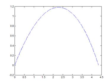
I actually wasn’t even looking at the online calculator you posted. Instead, I’m working with the Wikipedia equations. The initial conditions are as I posted before. Here is what I got: https://vexforum.com/attachment.php?attachmentid=9345&stc=1&d=1431823220
That plot is actually two lines pretty much perfectly overlapping. One is found from the following equations on the Wikipedia page:
The other is made by ODE45.
The using those above equations, the x position when y is zero is: 4.351450739677710
From ODE45 the x position when y is zero is: 4.351465250682764
However, calculating the range using the equation from Wikipedia yields: 4.387406051787434
The equation for this is:
Do you see the problem I am having? It’s not a huge difference, but the range should match up with the first two better than it is. I’ve looked over the range calculation multiple times and can’t find any problems, but I guess I must have made one. It’s not a problem because I am only really concerned with the accuracy of the ODE solution. I am just looking for a sanity check.
That’s interesting, when I work through it by finding t_ascend, t_descend, then the total time to work out total distance I get the same 4.387… value as the Range formula gave.
Are you able to work out the values for t_ascend, t_descend and maximum height for either of your first two methods? The values I work out are below:
t_ascend: 0.48651476336167 seconds
max height: 1.1822169506838 metres
t_descend: 0.4953908168235 seconds
Would be interesting to see where exactly this difference occurs
Upon further testing, I managed to get a value of 4.3514528749742 metres, which sits between your first two values.
I got this by setting the total time to 2 * t_ascend, rather than t_ascend + t_descend. Because of the air resistance the curve is asymmetric with respect to time and I’m wondering if that’s your issue.
Did you use both of the s_y(t) equations (one for up, one for down) in your calculations? You only listed the one for going down in your post, so just curious.
Essentially, you just leave one field blank in the calculator (launching speed is now editable) and it will fill it in for you automatically. And yes it will even work for X position, Y position, or launcher height (in case anyone ever wanted that… :p)
Hmm, so at this point I am going to abandon trying to recreate the analytically model in MATLAB and instead focus on the ODE45 model. I was only doing the analytically model to check the ODE45 results, but now that you have verified the range along with peak height and time I can use that.
I just wanted to check, what values did you use to solve for that range (Cd, density, etc)?
Here is the model I am using for ODE45. It requires you to give it a set of differential equations and initial conditions. Here is what i am using:
You plug in dY/dt into ODE45 along with the initial conditions and time frame and it solves it using the Runge-kutta method with 5th order error control.
Looking at my ODE45 results (I may have had gravity = 9.806 before, it’s now 9.81):
Ascent Time = 0.486500000000000
Descent Time = 0.486532482025582
Time of Flight = 0.973032482025582
Peak Height = 1.182193046366098
Range = 4.351450739677710
I am expecting some difference between the ODE solution and the analytically one. Somewhere in the range of tenths to hundredths of a percent seems fine. But I think a difference of 0.82 percent is quite a bit… If you would look over my above equations I will spend the meantime looking into tightening up the tolerances on ODE45 and maybe switching to a different ODE solver in MATLAB.
Upon writing this all out, I think I may have caught a mistake of mine, but I am not sure. I think the second equation should instead read:
Before, I was squaring the x velocity and y velocity separate to get the drag force in the corresponding direction. I am pretty sure that is wrong. With it corrected, I am solving for the drag force using the total velocity and then using the angle to find the x and y force components.
This all sounds right to me, but the problem is that when I reran the program the results were even farther away from the analytically data:
Ascent Time = 0.473400000000000
Descent Time = 0.491568092149209
Time of Flight = 0.964968092149209
Peak Height = 1.142837679832881
Range = 4.256366726320169
That’s now a difference in range of 3 percent…
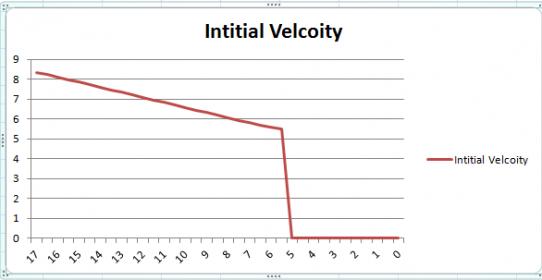
I used the spreadsheet I made to calculate the required launch velocities for a bunch of distances, from 17ft to 0, taking measurements every half of a foot
attached is the image of the graph it forms, and, you will notice the plots form a perfectly straight line, how could this be a linear relationship, and if it is truly linear, why all the fancy equations?
also, if it is not truly linear, could one write a linear approximation of it that would be close enough that we don’t care?
the sharp drop to zero is where the equations become impossible, essentially where that shot cannot be made a t a 60 degree launch angle
so I calculated the linear regression of the line, and then plotted it in reference to to the calculations out of the spread sheet, and got a differences of up to 5 Cm/s in terms of Vo, so it’s no good for getting an actual answer, but it makes a really good first guess for not program solving numerically for the answer, and is a lot simpler than the equations I was using before
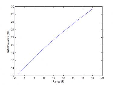
So I don’t think that graph looks correct. The graph should be fairly linear, but not exactly. Here is my plot. This data is for a ball launched 18in from the ground at a goal 36in tall. https://vexforum.com/attachment.php?attachmentid=9347&stc=1&d=1431891968
Notice how much larger my initial velocities are? With out knowing what kind of model you are using (are you including drag?) I can’t tell you what the problem may be. It is quite possible though that mine is wrong. You could approximate the relationship between initial velocity and range to some degree. However, it looks like this breaks down for short shots.
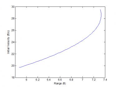
The linearity can also break down when you induce spin on the ball. Here is a clearly non-linear plot for a ball with a constant 80 rpm backspin. https://vexforum.com/attachment.php?attachmentid=9348&stc=1&d=1431891974
It’s from a Kutta/Wagner model I am working on now. Notice how there is actually a maximum range? These are the things I’m trying to find.
I do have a good reason for all these equations. As we start making fewer and fewer assumptions (and take into account more factors, say the spin of the ball), the model governing its flight becomes more complicated. It gets to the point where there is no analytical solution to the problem and we have to instead use numeric methods to solve it. I am trying to make sure the numeric methods solution match the analytic solution with the simpler models so that I know the results from more complex models are correct.
EDIT: Actually, I think I see the problem I had with the graph you showed. The range is measured in feet and the initial velocity is in meters per second, isn’t it? If that’s the case, the plot looks correct. Although, because the important data is scrunched up you cant’t really see the slight curve.
your assumption is correct, the bottom line is in Ft, and the top in meters, and I have noticed the curve, when I plotted the error, and multiplied it by 100, you could really see it, but because the range of our equation is so short, 0 to 17 ft, the equation is close to linear, at the edges of the graph the error would cause the landing distance to be about 5 cm off.
I am solving for Vo numerically and my quest has been to get the required number of iterations down as low as possible, so first I just added part of the error to the velocity to be tested in the next iteration, and i just started all my guesses at 10 m/s. it then took 11 iterations to get below 1 cm of error, next I analytically solved for Vo in an equation not counting for drag and used that number as my first guess, that got my error down to less than 1 cm in 3 iterations, and using this new linear model as my first guess, I got it down to 1 iteration, I use the linear model as my first guess, make on correction and it is less than 1 cm error for anything between 0 and 17 ft