the shooter my team is making will absolutely induce spin to the ball, could you tell me how to calculate for spin, what are the relevant equations, and how does spin factor in. spin was not in the wikipedia page posted here. also, what in heck is a kutta.wagner model?
Short answer: It’s complicated. The trajectory of a rotating sphere is a function of air conditions, velocity, heading, distance traveled from impulse, rate of rotation, and various initial conditions.
Really long answer:
I started with the simplest projectile model (no drag) and have been adding on components one at a time. Now one thing you should realize is that I am not solving these analytically. I am using a numerical differential equation solver on the computer. You give it a set of governing equations (model) and some initial conditions, and it solves for the trajectory sort of how you might integrate acceleration over time to get a robot’s position on the field, except it is much more accurate :).
My next step was to include drag on a smooth sphere based on a constant coefficient of drag (.47) like nallen has done. My data didn’t match his to the degree I would like, so I may have made a mistake here. If so, I can correct it very easily once I figure out the problem.
Regardless, I moved on to a model that included drag with a varying coefficient of drag. The drag will increase when the speed of the ball drops significantly. This didn’t have much affect on the cross-court shot (it decreased the range by about 0.25 inches), but it had a larger effect later when I included lift due to spin.
Here is where the Kutta part of the model comes in. Lift on a cylinder is predicted by the Kutta-Joulowski theorem. It predicts the lift on a cylinder as a function of the circulation of flow around it as well as its velocity through a fluid and the fluid conditions. This translates to a certain lift force generated by back-spin on the ball. However, this lift force is tangent to the direction of travel (not straight up) which complicates things a little. Also, a top spin will induce a negative lift force. Both of these can cause some crazy things to happen when the spin is increased. I’ve plotted trajectories with multiple loops ![]()
Now for the Wagner part (pgs 11-12). The Kutta-Joulowski theorem assumes steady state flow conditions. Wagner figured out that the lift generated by any airfoil subject to a large impulse in the flow parameters experiences a lift penalty for a certain distance. This gives us a nice quasi-steady state solution. What this means is because the ball has suddenly accelerated from 0 to our initial velocity, the lift due to spin begins at about half of what Kutta predicts and increases according to Wagner’s function where it will be 90% of Kutta’s lift after it has traveled 7 chord lengths (diameters). This requires us to treat the ball as a thin airfoil. It isn’t so Wagner’s function will be wrong to some degree, but I think including the lift penalty is better than not doing it.
And that is where I am at. I am still going over all of my model equations to make sure I didn’t make any silly mistakes before I let everyone pick through it. I am also trying to think of anything else I can include to improve the model. I’ve been digging around some old naval papers online looking for a good quasi-steady model for drag on a sphere without any luck. I’ll even just take experimental data at this point. I want to say that it would be similar to Wagner’s function on Kutta’s lift, but I haven’t found anything confirming that yet.
Anyways, here’s a nice little trajectory plot of a ball shot straight up from a height of .4572 m (18 in) at a velocity of 9.46 m/s with a constant top spin of 382 rpm at a goal 2 m away 1 m high.
https://vexforum.com/attachment.php?attachmentid=9349&stc=1&d=1431917511
The amount of spin is unrealistic in my opinion, but the plot is neat. I’m wondering if there is anyway I can predict how the spin will decay over the duration of flight as I know it isn’t really constant.
Here is a good example of the affect of the Kutta-Joulowski theorem and how much spin can have an affect on the flight of a ball. Notice the angle the ball is coming in on the table from yellow’s looping shots?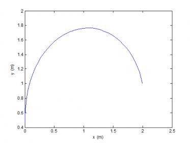
Nope, the way you had it first is the correct way. But you don’t even need to do work out Vsin(theta) or Vcos(theta) because Vsin(theta) = dx/dt and Vcos(theta) = dy/dt.
Doing that means you don’t even need your V and theta equations either.
Regardless, there’s still only one vertical equation you’ve got there when you should have two? One for going up and one for coming down since the direction of the drag force is different in each case.
I am pretty sure the way I had it first is still wrong. The drag force of the ball should be independent of the coordinate system we establish, right? So say we have a ball traveling at 4 m/s and k/m is a constant of 1. Well then we can say that the drag force is going to be 144=16 N. Now say we establish a coordinate system such that the ball is traveling 45 degrees relative to the x axis. We can decompose that drag vector into its components of 16/sqrt(2)=11.3 N in the x direction and 16/sqrt(2)=11.3 N in the y direction.
Now let’s try to solve for the drags using the x velocity and y velocity separately. Our ball is moving at 4 m/s at an angle of 45 degrees. That means the x and y velocities are both 4/sqrt(2)=2.828 m/s. If we solve for the drag it will be 12.8282.828=8 N in each direction for a total drag of sqrt(88+88)=11.136 N. See how decomposing the velocity vector before calculating drag causes a problem? It’s because the total drag force is a function of the total velocity squared. If it were linear there would be no problem decomposing the velocity vector first.
EDIT: It may help clarify the next part if I point out that theta is the angle of the instantaneous velocity during flight (the ball’s relative heading). It is not the initial angle that the ball is launched at, except at t=0 of course.
I am not sure why there should be two differential equations in the y direction? I understand why the analytically solution may have a piecewise aspect to it. However, Y[4] is the y velocity so dY[4] would be the acceleration in the y direction. Newton says this should just be a function of force and mass. The mass is constant, so the only reason I would need two equations would be if the force equation changed. I don’t think it does that. If you look at Y[4] I am taking the sin(theta). So as the relative heading of the ball becomes negative (theta changes to negative), the direction of the drag force will have a sign flip. If I were to put the cos(theta) inside of the square this wouldn’t be the case because the square would kill the negative sign. But with it outside I believe it is correct.
Your maths is wrong (drag components would be 16/sqrt(2) = 11.3N, x and y velocities 2.83m/s, combined drag 11.3N) but your logic is correct. I see your point and you’re right…
This means that all the equations we’ve been using are incorrect, I don’t even know if it would be possible to create equations for v_y, v_x, s_y and s_x now ![]() That makes it a bit harder…
That makes it a bit harder…
You’re right, I hadn’t had my morning coffee yet ![]() I’ll edit it with your corrected values.
I’ll edit it with your corrected values.
It is possible that you can’t do it, but I wouldn’t discount the idea completely. I’ll look into the MATLAB function dsolve later tonight to see if I can get an analytically solution to the model using symbolics…There is a chance it will work, but it’s slim.
Since I think I have the IVP down, I have been trying to set up the BVP problem (to solve for the initial velocity or angle of the launcher given a range). One problem I am having is that the stiffness of the ode model when you include spin is just whack. Another is that I can solve for the initial velocity given an initial angle and some restricting conditions (no wild loop de loop spins and such) over a large number of iterations (up to 200 sometimes ![]() ), but I can’t solve for the launcher angle given an initial velocity. With spin, the range of a shot varies wildly as you change the angle to the point that it just refuses to converge no matter what my initial guess is. I am really just not happy with how fussy the program is, it likes to diverge more often than converge.
), but I can’t solve for the launcher angle given an initial velocity. With spin, the range of a shot varies wildly as you change the angle to the point that it just refuses to converge no matter what my initial guess is. I am really just not happy with how fussy the program is, it likes to diverge more often than converge.
If I can’t get the BVP working, I guess I will just have to create a lookup table by solving the IVP over a range of initial angles, velocities, and spins… It’s not ideal, but it should work I suppose.
ok, I was looking over the Kutta–Joukowski theorem equations and I cannot figure them out, at what point do they take into account the spin of the ball, I understand how they help if the ball may act as an air foil (maybe?) but there aren’t even any variables that take into account rotation. I see that there are equations that take into account the pressure differential between top and bottom, and that the differential could be caused from spin, but how does one calculate pressure differential based on spin.
also that wagner stuff just melted my brain, probably not helping that i have not taken any physics or calculus.
So the thing about Kutta-Joukowski, and most of aerodynamics for that matter, is that you treat your airfoil (ball) to be stationary and look how the flow acts around it. So when you use this theorem the ball isn’t spinning, but instead there is a flow circulating about the sphere signified by gamma. I did a little looking and found NASA’s page on the matter which should be a little more clear than the Wikipedia page. That’s the exact equation I am using. You have to be careful what units you use though. S will generally be in radians/s so you will have to convert to a more meaningful rpm if that’s what you desire.
Also don’t feel bad about the Wagner stuff. Its graduate level unsteady/quasi steady aerodynamics that I only stumbled across in my research. I roughly know the theory. I know why there should be a penalty applied to the lift initially in our case, but have no clue how the Wagner function was derived ![]()
ok next question, how would I convert a force in lb/ft, into an acceleration, or something that would actually fit into the equations I have to calculate trajectory.
realy here is my problem, the direction in which the “lift force” would be applied is constantly changing, because the velocity and angle of movement of the ball is changing, you would need to calculate this for ever instant wouldn’t you?
for my level what would be great is if someone could just point me in the direction of the equations that tell you that X and Y position of a ball at any instant, and take into account the starting conditions, drag and spin, I don’t know, maybe that equation doesn’t even exist.
You can use Newton’s Second Law of motion which says the Force=mass*acceleration and solve for the acceleration.
Yup, that’s what makes it a pain. Same thing goes for the drag.
Sorry, but there just isn’t a simple equation that you can plug numbers into and solve on your calculator. It requires the computational power of a computer in order to solve it in seconds as opposed to days by hand.
I’ve finished the solver and am now figuring out how I can port it to a more usable format. I really don’t know much about Java or other languages, so it may take a day or two depending on how much free time I get.
So I roughed out a program that will plot the trajectory of a ball given initial conditions. I haven’t had enough time yet to port it over to a nice and light environment. Right now, I have an executable (windows only, sorry) that requires the user to download and install the MATLAB runtime (800MB, again sorry ![]() ) to use it. The upside is that the program itself is only 1MB and that once you have the MATLAB runtime you would only need to redownload the little .exe if I change it or write other programs…
) to use it. The upside is that the program itself is only 1MB and that once you have the MATLAB runtime you would only need to redownload the little .exe if I change it or write other programs…
Here is the link to the MATLAB runtime installer. You need version 8.3 or higher.
Right now it is beta at best. This is my first attempt at creating a GUI in MATLAB and interfacing it with a function like this so it may seem clunky to use. If you input crazy velocities (100m/s), or spins (10000) it wont converge on the solution fast enough and won’t show you the final range. Also, make sure to note that everything is in metric units. Backspin (ccw) is positive, topspin(cw) is negative.
I think that is everything you need to know…tell me how it goes. I expect someone to break it before I wake up tomorrow morning ![]()
I will post the MATLAB code if desired.
The matlab code would be much desired ![]()
I haven’t been following all the details of whatever you guys are doing with your equations and so forth but this one little line just jumped out at me. Does this mean that your launching speed calculator which you posted on page one of this thread is no longer correct? ![]() Or are you discussing some other issue?
Or are you discussing some other issue?
Here is part of the code. I will post the rest tonight when I get home. This is the ode function which is the meat of the model. It gets called by one of MATLABs own functions, ODE45, where it is solved. You just have to feed ODE45 some initial conditions and tell it when to stop.
function  dY ] = ODE_DragKuttaWagner( t, Y)
global D rho g m mu spin

A=pi*D^2/4;

dY=zeros(5,1);

dY(1)=Y(3);
dY(2)=Y(4);

V=sqrt(Y(3).^2+Y(4).^2);
theta=atan2(Y(4),Y(3));
Re=V*D/mu;

W=1-.164*exp(-.0455.*Y(5)./(D/2))-.335*exp(-.3.*Y(5)./(D/2));

Cd=(777*((669806/875)+(1149746/1155)*Re+(707/1280)*Re^2))...
    /(646*Re*((32869/952)+(924/643)*Re+(1/385718)*Re^2));

dY(3)=(-0.5*rho*A*Cd*V^2*cos(theta))/m-...
    W*((4/3)*(4*pi^2*(D/2)^3*spin*rho*V)*sin(theta))/m;

dY(4)=-g-(0.5*rho*A*Cd*V^2*sin(theta))/m...
    +W*((4/3)*(4*pi^2*(D/2)^3*spin*rho*V)*cos(theta))/m;

dY(5)=V;
ODE45 plugs your initial conditions into this as vector Y and uses the output vector dY to integrate it over a very short time step. It takes the new conditions after integration and repeats this over and over till the ball hits the ground.
Y1 is the x position, Y2 is the y position, Y3 is the x velocity, Y4 is the y velocity, and Y5 is the arclength of the trajectory. All of the values are instantaneous at the point of integration (i.e. the arc length is the measure of the distance traveled by the ball up till the integration point).
I apologize that the code is so messy and isn’t commented. It was on the list of things to do last weekend that I didn’t get to.
Also, W is the Wagner function and Cd is the coefficient of drag function that depends on the current Reynold’s number. Reynold’s number is an aerodynamic parameter that is dependent on air conditions, object size, and speed. The globals at the top are stuff that you define outside the program before hand.
EDIT: For those that don’t know, ode stands for ordinary differential equation. For those without calculus backgrounds, it is sort of like an algebraic equation, except instead of finding what a variable equals, you find what the slope of the variable is…kinda confusing and hard to explain.
Unfortunately, yes ![]()
I’ll look at potentially getting it to work with this new knowledge but it’s much harder to implement…
Despite it being “not correct” it’s still more correct than no air resistance, and even should be more accurate than cv, but it’s not 100% accurate to the real world values (somewhere between cv and c*v^2)
Nathan, if I were able to take the MATLAB code I have now and generate just a huge array of data from it, would you be able to integrate that into your calculator?
I could iterate the code with each parameter changing, say velocity from 1 to 10 m/s, angle from 5 to 85 degrees, and spin from -400 to 400 rpm with say 1000 points in each of those ranges (for a total data set of 1000^3 points…) and output it along with the corresponding shot range to an excel file, or whatever you like.
Then on your end you would modify your calculator so that it took the user inputs (range, spin, etc.), looked for the data point that closest matched these (it may have to extrapolate or just use the nearest point since there will be discrete data points and the user may choose a value between ones that have been calculated) and reported back the missing parameter they need.
I know it isn’t ideal and I am really not sure how much data is too much (it may take a while to iterate the solver that many times, but I can run it while I am at work one day), but I think it could work.
In an ideal world where data isn’t an issue, I could also give you the xy data and you could show a trajectory plot with the solution. The only problem I can think of is that there may be multiple solutions for each range even with the other parameters pre-selected. When you set your backspin high enough the ball will loop at some speeds and not others so you could have two speeds with the same range… I could figure a way to remove all the data points that involved loops before hand though if that helps.
1000^3 data points… well, that’s a lot.
so if I understand this, the equations on the wikipedia page are incorrect as a result of an error in the calculus equations from which they are derived?
I was going back and looking at the posts in which you described the error, and you described that if the ball is traveling at 45 degrees, force in x and force in y directions = Sqrt(Total force/2) how can this be true, if this were true then if we summed the X and Y forces, we would get less than the total force we started with. I believe in the example you said we started with 16N of force total, and when we decomposed it we got about 2.8 newtons in x and in y, for a total of about 5.6, but we started with 16 newtons
you also say that if we were moving at 45 degrees at 4m/s we would be moving and 4/sqrt(2) in X and Y, but then we have the problem that if we add velocities of x and Y we get more than 4m/s in total.
I believe my confusion here is caused by a basic misunderstanding of physics, if i have a projectile traveling at 45 degrees, do the X and Y velocities not split to two equal parts? does this have something to do with SIN(45) equaling 2/Sqrt(2) and if so, then how can it be possible that adding Vx and Vy would sum to more the Vo